Growth or cannibalization? Success or failure of promotion?

Promoting a product, especially one that involves a reduction in its price, almost always results in an increase in sales. But does every increase mean that the promotion was profitable? How often does the promoted product take customers away from other substitute products? How to calculate how much is the actual “incremental” of the action?

The fundamental question to solve the problems identified in the introduction is: what if… Or more precisely: what if there were no promotion. How much would the sales of the promoted product have been? How much would other products (especially substitute products for the promoted one) have sold? On the surface, this seems impossible to determine. After all, we are asking about an alternative reality that we are unable to observe. It is impossible to introduce a promotion and not introduce it at the same time. However, it turns out that based on advances in statistics, data science and artificial intelligence research in recent years, we are able to estimate the aforementioned effects in a scientific, methodical and rigorous manner. The method used is based on so-called synthetic control groups. That is, to put it somewhat simply, comparison groups created by a special algorithm on the basis of available observations of sales of similar products.

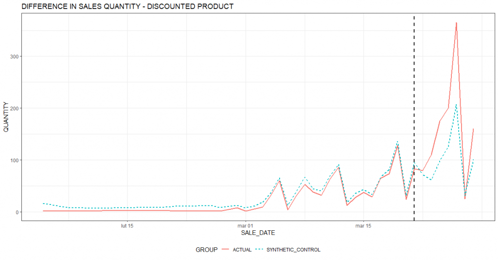
We will analyze this using the example illustrated in the chart below. The red line shows the actual sales of the product (in units). You can see that before March, sales of the product were traceable. You can also see a clear weekly cycle with peaks on Saturdays and clear declines on Sundays (related to the trade ban and the limited number of outlets that can conduct sales). One can also see an upward trend in sales since the beginning of March. The black vertical dashed line shows the day the promotion started. The price of the product has been significantly reduced. A clear increase in sales can be seen.
kanibalizacja

The light blue dashed line is the algorithm’s estimated sales behavior of the promoted product if there were no promotion (alternative reality). It can be seen that even without the promotion there would have been an increase in sales (in line with the upward trend visible since the beginning of March). However, it would not have been as large. Therefore, it can be concluded that the promotion generated additional sales of the product.

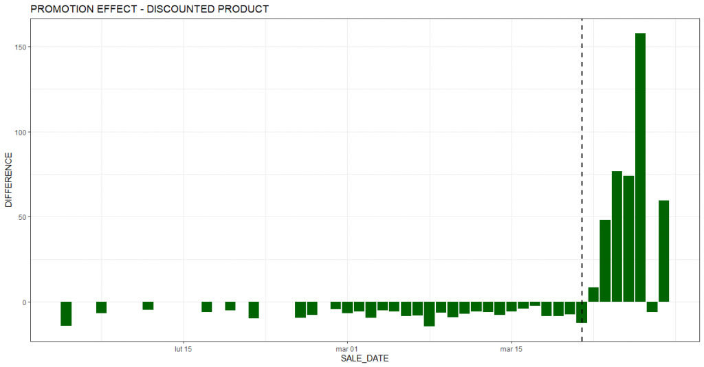
The next chart shows a summary of incremental sales for each day. As in the earlier chart, the black vertical dashed line marks the beginning of the promotion period. Most of the bars are clearly above zero, indicating an estimated increase in sales relative to the base scenario (i.e., no promotion). The period preceding the promotion to the left of the dashed line is the calibration period. Based on this period, the algorithm learns the best combination of products that make up the comparison group (the so-called synthetic control group). The closer the bars in the calibration period are to zero, the better the matched comparison group. Of course, in real-world examples (such as the one presented in this article) it is difficult to find a perfect match. Hence, the bars deviate slightly from 0. What is important, however, is that the magnitude of these deviations is much smaller in the calibration period. This lends credence to the conclusion of a real positive effect of promotions on sales.
efekt promocji

At this point, one could close the analysis and congratulate those responsible for the promotion. The question arises, however, to what extent the promotion attracted new customers or increased demand from existing ones, and to what extent it merely shifted demand from other complementary products that were not promoted during the period. In other words, to what extent did the promotion scanibalize sales of other products.

To answer this question, we will conduct a similar analysis to the one presented above. This time, however, the red line will represent sales of a substitute product to the promoted product. For this particular product, we want to estimate the cannibalization effect.
różnica w sprzedaży

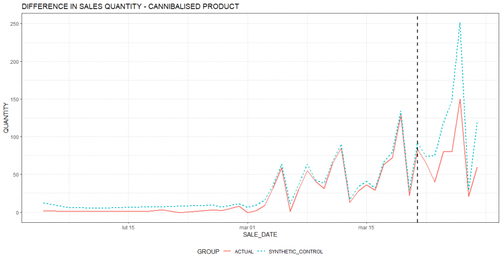
As before, the vertical black dashed line marks the date of the start of the action. After the start of the promotion, the red line is lower than the light blue dashed line, which means that the substitute product is sold less than it would have been sold in the baseline scenario assuming no promotion. It is also worth noting that in the period before the promotion (the calibration period) the two lines are very close to each other, which means that the algorithm has correctly calibrated the comparison group.

The chart below summarizes the effect of cannibalization by day. You can see that on each day of the promotional period the product sold less compared to the reality that the promotion would not have taken place.
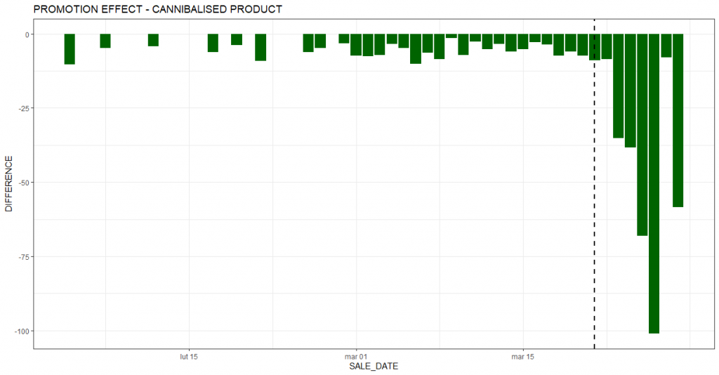
In the case analyzed, the incremental sales of the promoted product amounted to 407 units. However, when evaluating a promotional action, one must take into account the effect of cannibalization. In this case, the loss of sales on a product substitutable to the promoted product amounted to 326 units during the promotional period. Without taking this factor into account, we could significantly overestimate the financial effect of the action and draw incorrect conclusions as to its profitability. This, in turn, could translate into suboptimal decisions on organizing similar promotions in the future.

The best way to measure effects is to conduct a randomized experiment. However, this is not always possible. It is difficult to imagine how to run a promotion and not run it at the same time and for the same group of consumers. In such situations, modern analytical methods based on synthetic control groups, among others, such as the one presented in today’s article, can be invaluable in marketing analysis.


Prediction and segmentation as weapons in the fight against churn

Customer churn is one of the key challenges facing organizations in today’s highly competitive environment. In order to effectively combat customer churn, companies need to find answers to two key questions: which customers are at risk of churning, and what actions can be taken to stem the process.

With help comes a combination of two methods from the arsenal of data science: prediction and clustering (segmentation), which together increase the effectiveness of retention efforts.

I have already addressed the issue of prediction of the threat of customer churn in an article in the We Love Data So Let’s Date series. Due to the importance of the topic and the interest it has generated, I decided to deepen the issue and present an approach in which, by combining two machine learning methods, we can significantly facilitate the implementation of data-driven anti-churn activities.

Prediction and segmentation as a weapon in the fight against customer churn

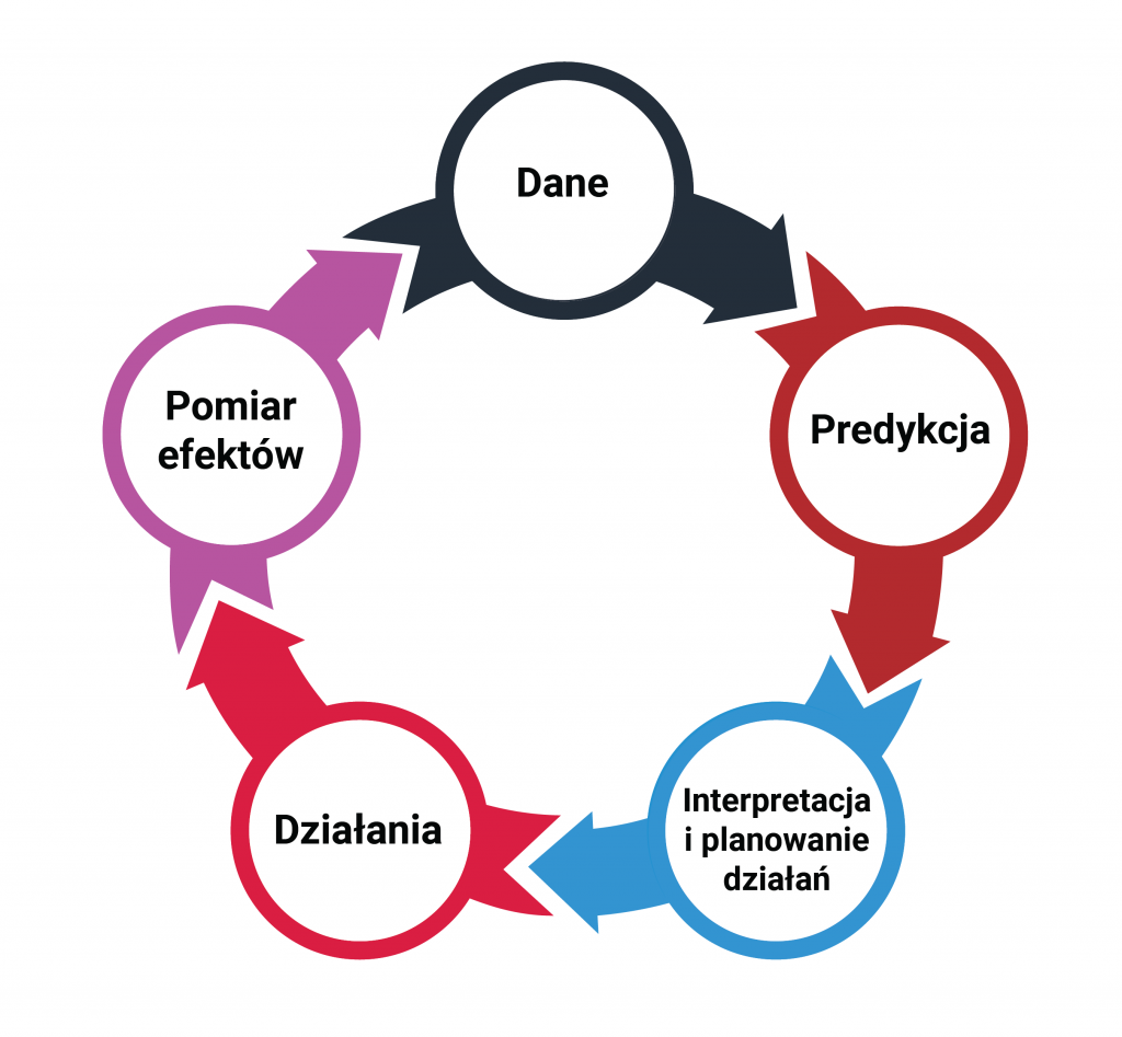
The basic tool in countering customer churn is the predictive model. It allows predicting the probability of a particular consumer leaving. However, this may not be enough. Even the best model and the most accurate prediction will be of no use if we do not take appropriate action based on the information received.

Proper interpretation of the data allows us to plan activities and take actions – such as sending an sms message to customers or offering a discount on selected products. We then measure the impact of the action (effect) on consumer behavior and their propensity to abandon further use of the offer. Measuring and observing consumer behavior provides a source of new data that the predictive model can use. Thus the cycle closes, and this is illustrated in the diagram below

The predictive model indicates the likelihood of a specific customer churning. This allows us to prioritize tasks and use the usually limited resources on consumers most at risk of leaving. Information that a consumer has a 75% probability of leaving within the next quarter helps us decide that “something” must be done about it quickly. However, does it provide the knowledge of what to do? How does a company know what action to take? The key is to interpret the data correctly.

The ideal situation would be to be able to take action personalized to the individual consumer. That is, each customer would receive a unique customized offer tailored to their needs and problems. Predictive models built on the basis of appropriately selected machine learning methods make it possible to create an individual profile of each consumer. In addition, they indicate specific factors that in his case are associated with a higher risk of leaving. Despite advances in the area of hyperpersonalization of marketing activities, it is still not yet achievable on a large scale for many organizations. Not all activities can be automated as easily. For example, creative, content production or offer construction can be a limitation.

The solution in such a case is an approach based on advanced segmentation. However, it is definitely not about classic segmentation, which uses only basic variables like age or gender. They do not sufficiently differentiate the base, and the real dividing lines run quite elsewhere. It is important, therefore, that it be a behavioral segmentation, in which we look for similarities in customer behavior, taking into account the same broad aggregate of descriptive variables that was used to build the predictive model. In order to perform such a comprehensive segmentation, clairvoyant machine learning algorithms are required.

The procedure may look as follows:

  1. The predictive model allows us to identify the group of customers most at risk.
  2. We decide that we have the resources to act against the 20% of the most at-risk customers.
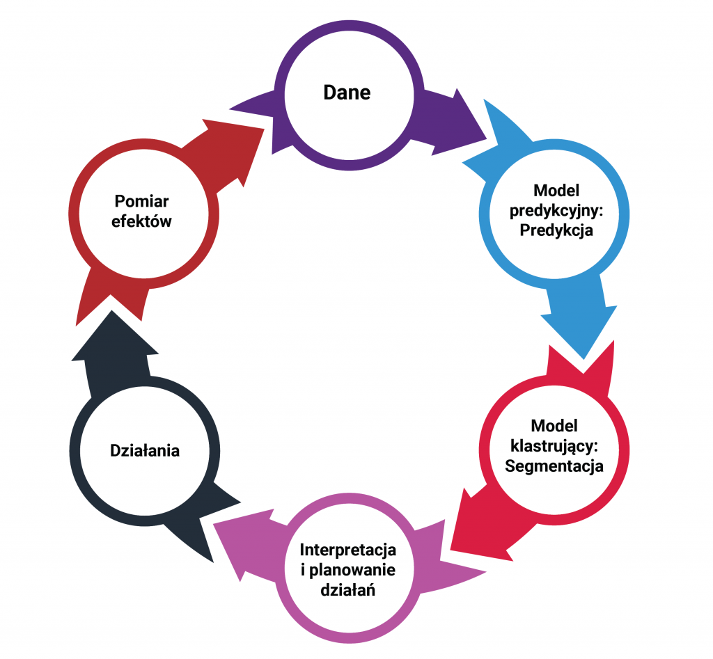
  3. We select these customers and, using a clustering model, divide them into segments. Their number should be a product of the model’s indications and the resources we have to serve them (usually it will be several – a dozen).
  4. We interpret the segments and plan actions.

The proposed method makes it possible to put into practice predictive modeling and the in-depth understanding provided by data science analysis of consumers at risk of leaving. The approach will also find application in companies not yet technologically and organizationally ready for fully automated hyperpersonalization efforts.

.

How do you count the campaign effect so that you can (almost) always declare success?

After a campaign has been carried out, marketers wonder whether and what kind of profit their action has brought. Summarizing the projects completed so far and planning future actions, they try to find the answer to this nagging question. They calculate the effectiveness in various ways. Usually, the greater the effect, the less inclined they are to reflect on whether their method of calculating efficiency is at all correct. Add to this some obvious, but still frequently made mistakes, and thus overinterpretation of the results is guaranteed. So is there a foolproof way that makes it clear how the effect of an action should be calculated?

Misjudging the effect of the action

Here is a simple example to illustrate the idea. Suppose we organize a campaign, rewarding all customers who have agreed to receive marketing e-mails. Everyone we can contact in this way will receive by e-mail a discount voucher for the amount of PLN 20. The idea meets with approval. The selection criteria are simple. The action is quickly implemented. So fast, in fact, that there was not enough time to think about how its effect would be measured. Somehow, however, it would be appropriate to measure it. After all, one can make a comparison of sales in the group that received the coupon to the group that was not qualified for this action. Well, that’s just it. After all, it’s simple.

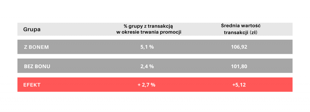
Wykres porównawczy grupy z transakcją do grupy bez transakcji

With a base of 100,000 consumers, we generated 2700 additional transactions (2.7%100000 = 2700) and increased the value of 2400 transactions by PLN 5.12 (2.4%100000 = 2400). Thus, the total turnover generated was 301 thousand zlotys. The cost of the vouchers used was 102 thousand zlotys (5100 * 20 zlotys = 102000).
So success. Is it?

Such a solution is very simplistic. In fact, one could even use the term naive, and it distorts (usually overstates) the incremental effect of the action. This is because the above method of calculation ignores one important detail. The groups being compared are different from each other, and not just the fact of receiving a voucher. The group with the voucher receives e-mail communication, while the group without the voucher simply does not receive such communication. The assumption that the group that has consented to e-mail communication will be more likely to make purchases, even if it does not receive a voucher, is plausible. If we assumed the opposite, it would mean that communication has no effect on sales, yet we know that this is not the case.

First: plan in advance how to analyze the effects

So what to do in this situation? The best approach, would be to plan how to analyze the effects even before launching the action. That way, an appropriately sized control group could be drawn from among all customers who meet the criteria. This group would not receive a voucher. This would be the only significant difference from the group receiving the voucher. This would make the control group a better and more reliable background for comparison. A similar campaign was indeed carried out for one of our clients, but its effects were measured correctly. Even before the mailing, we selected the appropriate volume of the control group from among those with consent to communicate via email. The results of the correct comparison can be seen in the table below.

Wykres porównawczy transakcji osób z bonem do osób bez bonu

We can still see a positive difference in the percentage of the group with a transaction. However, it is much lower in the case of the previous comparison and is only 0.8% According to the new estimates, we generated 800 additional transactions (0.8%100000 = 800) and increased the value of 4300 transactions by PLN 7.79 (4.3%100000 = 4300 transactions). As in the previous case, the cost of the used vouchers amounted to 102,000 (5100 * 20 PLN = 102000). Thus, the total turnover generated was 119 thousand zlotys (85.5 thousand zlotys + 33.5 thousand zlotys). So it was not much higher than the cost of the discount given in connection with this action. So it is difficult to declare success. However, conclusions should be drawn and appropriate changes should be made when planning future actions (e.g., better selection of the value of the discount, adoption of other criteria for the selection of customers). However, should one also conclude that the described method – an experiment based on random control groups (also called A/B testing) – must always be used for this kind of analysis? Yes, but…

What if a control group cannot be distinguished?

Unfortunately, this approach is not always feasible. And this is its main drawback. There are legal constraints in certain situations (e.g., regulatory interpretations that limit the ability to discriminate against customers and mandate that benefits be given to all who meet certain criteria), as well as marketing constraints. For example, a company may not want to run the risk of causing dissatisfaction among customers who are cut off from benefit opportunities as an experiment. The risk is greater the higher the value of the benefit in the eyes of customers. So in such situations, are we doomed to a falsely simplistic approach or must we abandon analyzing the effects of a marketing action altogether?

Who are the statistical twins?

Not necessarily. Fortunately, we do not have to assume such drastic scenarios and give up on measuring the effects of the campaigns carried out. There are advanced statistical methods that allow even without a control group to estimate the actual effect. These methods, to put it simply, are based on the search for statistical twins. Statistical twins are customers with as similar characteristics as possible, among whom only one was subjected to an incentive: he was covered by a promotion, we sent him a text message, displayed an online advertisement to him, or took other actions towards him to encourage him to use our offer. This creates a synthetic “control group” consisting of one twin from each pair, the one who did not participate in the action. The challenge in this case is to identify the key variables that guarantee the similarity of the groups. However, appropriate computer software helps carry out this process. This opens up new possibilities for analyzing data and optimizing decisions in situations where conducting a randomized experiment is not possible, or is difficult or uneconomical.

As we can see, it happens that the effects of marketing campaigns carried out are either miscalculated or the results are overinterpreted. Therefore, even before implementing a campaign, it is necessary to determine how we intend to study its effects. Advanced statistical methods and machine learning help in many problematic situations, such as the inability to compile an optimal control group.

Seasonality vs. product pricing. How to price a product to sell and make money?

Setting the correct price for a product or service is one of a retailer’s biggest, and most important, challenges in a competitive market. A price that is too low reduces revenue and, consequently, profit. Conversely, a price that is too high reduces demand and also reduces revenue. While the unit profit on sales is higher, it may not offset the losses associated with reduced volume.

Determining the optimal product price – where to start?

The difficulty in determining the optimal price of goods is due to the number and complexity of factors that affect it. These include the prices of complementary and substitute products. To the list can also be added promotions, advertising, the activity and offerings of competitors, the economic situation of customers, their tastes and preferences, the cost of purchasing goods, logistics issues. Additional challenges are associated with products whose demand is seasonal and is due to weather conditions, for example. A classic example of such an assortment is ice cream, the demand for which is closely related to the air temperature. Other such products that can be mentioned are sunglasses, skis, cool drinks, winter jackets, swimwear, hotel services, tourist flights.

The paradox of price

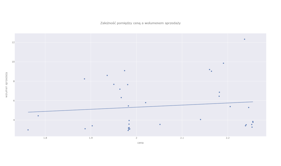
There is often a price paradox with these types of products. The classical economic theory of supply and demand says that the higher the price, the lower the demand for a good or service. This is usually the case. However, in the case of eminently seasonal products, this relationship can be shaken. After all, it often happens that the highest prices are quoted during the peak season for a given product. That is, when sales are highest as well. Sellers, knowing that it is during this period that consumers most need the product and are most likely to buy, take advantage of this by raising prices. A situation of this kind is illustrated in the chart below. You can see a gentle but clear positive relationship between price (horizontal axis) and volume sold (vertical axis).

Zależność pomiędzy ceną a wolumenem sprzedaży

Just looking at this graph, which is essentially a simple price-demand model, one could draw the naive conclusion that raising prices increases sales. As we know, this is not true (except for a very narrow and specific group of luxury goods). By raising the price of ice cream between October and March, we will not succeed in increasing its sales.

The relationship observed in the graph is the result of the intertwining of two factors. First is the effect of price and air temperature on sales, and second is the effect of temperature (season) on price. The latter is precisely related to the seller’s decisions to adjust the price to the increased demand.

Is there an ideal price estimation tool?

Thus, solving the puzzle of the real effect of price on sales requires a somewhat more complex approach than the analysis of the correlation between price and demand (an example of which was illustrated in the previous chart). Randomized experiments (e.g., A/B tests) are the ideal tool for estimating such effects. In theory, one could imagine that a retailer would randomly change prices so as to test different variations and combinations – resulting, for example, in an increase in the price of ice cream in December, or its drastic reduction in an exceptionally hot June. In practice, however, this is hardly feasible, and if only on a small scale and for a limited time. This is because it is a very expensive experiment.

Selling products at suboptimal prices drains revenue. In addition, frequent and unpredictable price changes can negatively affect consumers’ experience and induce them to switch to competitors. A practical solution, then, is to use the data we already have that are not from the experiment to estimate the effect of the factor of interest (in this case, price) on the outcome that is important to us (in this case, sales). It is possible, although it should be noted that this is not a trivial task and requires an elaborate mathematical apparatus. In today’s article, however, I will not focus on the mathematical, statistical and philosophical nuances involved in causality analysis. Instead, I will show the possible results of this kind of analysis and their practical effects.

Seasonality vs. product price

The solution requires at the outset the imposition of a “model” on the data that reflects our understanding of how the system we want to analyze works. This requires both common sense and expert knowledge. We can describe our assumptions using a graph, as illustrated below.

Cena produktu

First of all, as you can see, we set assumptions as to the direction of influence of the various variables. The price changes under the influence of temperature (or, more precisely, by the actions of the retailer resulting from his knowledge of the effect of temperature on consumer behavior). The retailer, on the other hand, by changing the price, is not able to change the air temperature – I think this is not a controversial assumption – hence the arrow points in only one direction. Temperature also has a direct effect on sales (when it’s warm more people are eager for ice cream). In addition, we take into account that other factors that are beyond our observation may also affect the price and affect sales. This is, of course, a very simplified model and can easily be expanded to include other factors that affect price or sales.

Estimation of the actual effect of price on sales

Based on such a formulated model and historical data on price, volume and temperature, using advanced analytical methods, it is possible to estimate the actual effect of price on sales. In other words, we can estimate to what extent a change in price is the cause of a change in sales volume. From there, it’s only a step to putting this knowledge into practice and optimizing the price.

The following example shows the process of finding the optimal price for ice cream in the month of September with a forecasted average daily temperature of 14.2 degrees C. We can generate similar charts for any temperature value, which is important in this case. This is because the optimal price will be different when September is exceptionally warm, and different when there are records of cold weather.

Wpływ zmiany ceny produktu na przychody ze sprzedaży - prognozowana średnia temperatura: 14.2

September is a transitional month between the peak season and the autumn-winter season. So far, the retailer has traditionally kept product prices still quite high in September. On the horizontal axis of the graph we show the change in price relative to the base price – this is indicated by the 0 line near the center of the graph. The blue curve shows how sales revenue changes depending on the price adopted. Moving to the right of line 0 (i.e., increasing the price), we observe a decrease in revenue. A higher price negatively affects demand, and higher unit revenue does not compensate for the decrease in will. Moving to the left of the 0 line, we observe an increase in revenue, although only up to a certain point. Beyond it, increased sales volume ceases to compensate for the drop in price. This point marks the point of optimal price – indicated by the vertical dashed line. The model suggests that the optimal price is 80 cents lower than the existing base price.

Following the recommendation and lowering the price results in an increase in turnover of just over 26% compared to the base scenario. This is illustrated in the chart below.

Przychody ze sprzedaży we wrześniu w zależności od scenariusza

The method presented in the article offers tremendous opportunities, using the latest research advances in artificial intelligence and causal analysis. In practice, of course, for greater accuracy, the model should also take into account additional factors such as prices of other products, prices at competitors, advertisements, flyers, newspapers, offers, promotions, macroeconomic factors. The full solution also gives much more in-depth insights. Simulating the impact of pricing decisions on sales volume and revenue helps you make better decisions. These, in turn, translate into measurable financial results and can give a significant competitive advantage.